'It's not like the movies, they fed us on little white lies': IMDb movie ratings
So, the Internet Movie Database (IMDb) has some nicely precompiled datasets that even seem to be updated on a daily basis. Let’s put them to good(?) use. We’ll use two files because the file with ratings only has unique identifiers that have to be merged with the actual names. I’ve downloaded these files before, so they might be a bit out of date. I am not doing this here, but it might be easy to modify the vroom() calls below to always get the up-to-date data gzipped files directly from the website.
library(tidyverse)
library(vroom)
library(scales)
library(hrbrthemes)
library(ggside)
library(ggeffects)
library(ggridges)

tit <- vroom("title.basics.tsv")
rat <- vroom("title.ratings.tsv")
First, some housekeeping:
- Only select movies
- Select movies with a runtime longer than 89 minutes and a maximum runtime of 4 hours (because, let’s be honest, who wants to watch a longer movie?)
- Select movies with publication year information
mov <- tit[tit$titleType == "movie",]
mov$runtimeMinutes <- as.numeric(mov$runtimeMinutes)
mov90 <- mov[mov$runtimeMinutes >= 90 &
               mov$runtimeMinutes <= 240,]
mov90$year <- as.numeric(mov90$startYear)
mov90 <- mov90[!is.na(mov90$year),]
Now, we’re merging the rating information (tconst is the unique identifier for each item) and removing all movies without an average rating.
mov90 <- merge(mov90, rat, by = "tconst", all.x = T, all.y = F)
mov90 <- mov90[!is.na(mov90$averageRating),]
How many ratings?
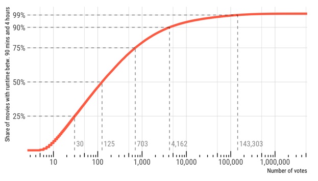
If we are dealing with movie ratings, we might want to decide how many ratings a movie should have to analyze it further. We can plot an empirical cumulative distribution function (ECDF) to get an impression of the number of ratings. I am inserting line segments at the quartiles and at the 90th and 95th percentile. The 90th percentile, for example, means that 90 % of all movies have fewer than this number. This number for the current selection of movies is 4,162.
qs <- c(.25, .5, .75, .90, .99)
ggplot(mov90, aes(x = numVotes)) +
  stat_ecdf(col = "tomato", linewidth = 1.5) +
  scale_x_log10(breaks = 10^(1:10),
                minor_breaks = 5*10^(0:10),
                labels = comma) +
  scale_y_continuous(labels = percent, breaks = qs, minor_breaks = NULL) +
  annotate(geom = "segment", y = qs, x = rep(0, length(qs)),
           yend = qs, xend = quantile(mov90$numVotes, qs),
           lty = 2, alpha = .5) +
  annotate(geom = "segment", y = rep(0, length(qs)), x = quantile(mov90$numVotes, qs),
           yend = qs, xend = quantile(mov90$numVotes, qs),
           lty = 2, alpha = .5) +
  annotate(geom = "text", y = rep(0.05, length(qs)), x = quantile(mov90$numVotes, qs),
           label = paste0(" ", comma(round(quantile(mov90$numVotes, qs)))), # pasting a space is a dirty hack to keep space to segment constant over log scale
           hjust = "left",
           family = "Roboto Condensed", alpha = .5) +
  labs(x = "Number of votes", y = "Share of movies with runtime betw. 90 mins and 4 hours",
       title = "Number of ratings",
       subtitle = "Empirical cumulative distribution function (ECDF)") +
  annotation_logticks(side = "b") +
  theme_ipsum_rc()
Alright, let’s make a totally arbitrary decision here: I’ll select the top 25 % of all movies (in terms of number of votes). The cutoff for this dataset is 703 votes.
mov90v <- mov90[mov90$numVotes >= quantile(mov90$numVotes, 3/4),]This leaves us with information on 37,709 movies.
Distribution of ratings
We are now plotting a histogram of these remaining movies. The little cross in the boxplot is the mean rating over all of these movies (6.3).
ggplot(mov90v, aes(x = averageRating)) +
  geom_histogram(fill = "tomato", bins = 30, col = "white") +
  geom_xsideboxplot(aes(y = averageRating, group = 1),
                    orientation = "y", fill = "tomato",
                    outlier.alpha = 0) +
  geom_xsidepoint(aes(y = 5, x = mean(averageRating)), shape = 4) +
  scale_x_continuous(breaks = 1:10, minor_breaks = NULL) +
  scale_y_continuous(labels = comma) +
  labs(x = "Average rating", y = "Number of movies",
       title = "Distribution of average ratings") +
  theme_ipsum_rc() + theme_ggside_void()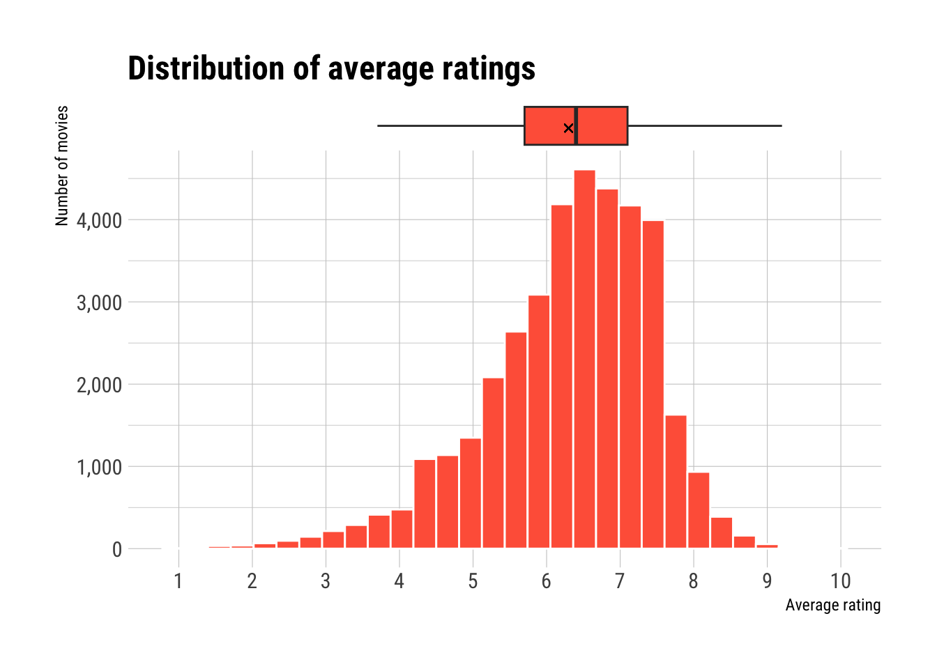
So, we have a lightly skewed distribution centered around the median of 6.4 and a mean of 6.3 but then rapidly falling of towards higher ratings. 50 % of all movies have a rating between 5.7 and 7.1. With a rating of 7.9 or above, a movie is already in the top 5 % of all movies. Speaking of top movies…
Top-rated movies
Let’s see our top 20 movies in this dataset.
mov90v %>% arrange(-averageRating) %>%
  select(primaryTitle, averageRating, numVotes) %>%
  head(20)
## primaryTitle averageRating numVotes
## 1 Nee Jathaga 10.0 739
## 2 Shubh Yatra 9.9 1319
## 3 Saachi 9.9 1224
## 4 Richiegadipelli 9.9 1206
## 5 Viratapura Viraagi 9.8 867
## 6 Suraari 9.8 762
## 7 Fuleku 9.8 1049
## 8 Yaadhum Oore Yaavarum Kelir 9.6 1142
## 9 Pichhodu 9.5 736
## 10 Youth Festival 9.5 769
## 11 Nodadha Putagalu 9.5 735
## 12 Chakravyuham - The Trap 9.4 2325
## 13 Killers of the Flower Moon 9.4 1371
## 14 The Shawshank Redemption 9.3 2751921
## 15 Jibon Theke Neya 9.3 2171
## 16 The Gilbert Diaries: The Movie 9.3 969
## 17 Maurh 9.3 1125
## 18 The Godfather 9.2 1914343
## 19 Ramayana: The Legend of Prince Rama 9.2 9945
## 20 National Theatre Live: Prima Facie 9.2 1268Interesting - I would be seriously impressed if you know any of those top 10 movies. Maybe our cut-off for the minimum number of ratings was a bit low. If we raise this to, let’s say, 100,000 votes, we get a list of usual suspects (The Usual Suspects (1995), btw, has an average rating of 8.5). But remember that, with this threshold, we are only looking at 1.41 % of all the movies in the dataset (n = 2,128) with a runtime between 90 minutes and 4 hours.
mov90v %>% filter(numVotes >= 100000) %>%
  arrange(-averageRating, -numVotes) %>%
  select(primaryTitle, averageRating, numVotes) %>%
  head(20)
## primaryTitle averageRating numVotes
## 1 The Shawshank Redemption 9.3 2751921
## 2 The Godfather 9.2 1914343
## 3 The Dark Knight 9.0 2724669
## 4 The Lord of the Rings: The Return of the King 9.0 1890626
## 5 Schindler's List 9.0 1387635
## 6 The Godfather Part II 9.0 1303631
## 7 12 Angry Men 9.0 815025
## 8 Spider-Man: Across the Spider-Verse 9.0 117525
## 9 Pulp Fiction 8.9 2113937
## 10 Inception 8.8 2418356
## 11 Fight Club 8.8 2191339
## 12 Forrest Gump 8.8 2140808
## 13 The Lord of the Rings: The Fellowship of the Ring 8.8 1919224
## 14 The Lord of the Rings: The Two Towers 8.8 1706369
## 15 The Good, the Bad and the Ugly 8.8 778663
## 16 Jai Bhim 8.8 207138
## 17 The Matrix 8.7 1961801
## 18 Interstellar 8.7 1917531
## 19 Star Wars: Episode V - The Empire Strikes Back 8.7 1323741
## 20 Goodfellas 8.7 1194446Top movies in decades
But wouldn’t it be also interesting to see which movies are the top-rated ones in their decade? Let’s do that. I am selecting all movies with more than 50,000 votes for this. We also have to shorten some titles to fit them in the plot.
# Select movies and annotate decade
mov90vp <- mov90v[mov90v$numVotes >= 50000 & mov90v$startYear >= 1930,]
mov90vp$decade <- paste0(substr(mov90vp$startYear, 1, 3),
                         "0s")

# Shorten some titles
mov90vp[mov90vp$primaryTitle == "Dr. Strangelove or: How I Learned to Stop Worrying and Love the Bomb", "primaryTitle"] <- "Dr. Strangelove"
mov90vp$primaryTitle <- gsub("Star Wars: Episode", "SW", mov90vp$primaryTitle)
mov90vp$primaryTitle <- gsub("The Lord of the Rings:", "LotR:", mov90vp$primaryTitle)

mov90vp %>% group_by(decade) %>%
  arrange(-averageRating, -numVotes) %>%
  mutate(rank_within = 1:n()) %>%
  slice_head(n = 10) %>%
  ggplot(aes(x = averageRating,
             y = tidytext::reorder_within(primaryTitle,
                                          -rank_within,
                                          decade))) +
  geom_point(col = "tomato") +
  tidytext::scale_y_reordered() +
  lemon::facet_rep_wrap(~ decade, scales = "free_y", ncol = 2,
                        repeat.tick.labels = T) +
  labs(x = "Average rating", y = "") +
  theme_ipsum_rc(base_size = 8)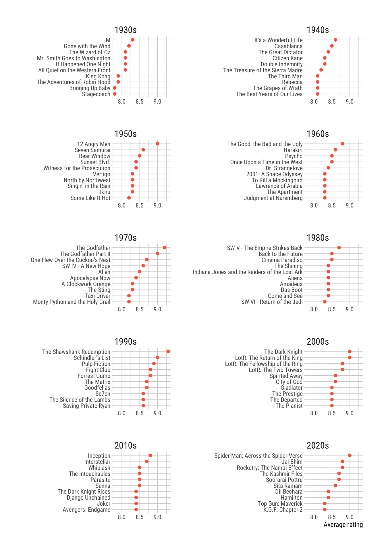
I have to admit: I have not seen a single top-rated movie from the 2020s. I would have expected Everything Everywhere All at Once (2022) in this list. As it turns out, its average rating is 7.8, so it’s not even close to the top 10.
Is there a “best” decade when it comes to movies? Let’s see…
mov90$decade <- paste0(substr(mov90$startYear, 1, 3),
                         "0s")
ggplot(mov90[mov90$year >= 1930,], aes(x = averageRating, y = decade)) +
  geom_violin(fill = "tomato", draw_quantiles = 1:3/4) +
  geom_point(stat = "summary", shape = 4) +
  labs(x = "Average rating", y = "",
       title = "Ratings in decades") +
  theme_ipsum_rc()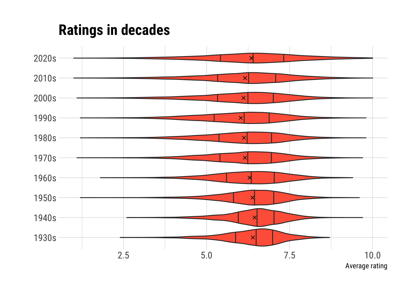
There’s certainly no huge effect going on here, and remember that these ratings contain all movies with a runtime between 90 minutes and 4 hours. It’s interesting to compare this plot with the one before: the top movies from the 90s are certainly shifted to the right (= higher average ratings). So, is it the mass of movies produced in the 90s that pulls its violin a bit to the left (in the plot above)? This might be something to investigate further in the future.
Best genres
But for now, let’s turn to genres. Things get a bit complicated because each movie can be associated to more than one genre. So, for plotting average ratings of genres, we let each movie count in every genre it is associated with. This is done in the code below. Also, we are concentrating on the top genres only, i.e. all genres that appear more than 300 times in the dataset of movies with more than 50,000 votes (and with a publication year after 1929).
# Most frequent genres, pick all that appear > 300 times
genres <- table(unlist(strsplit(mov90vp$genres, ",")))
genres_to_use <- names(genres)[genres > 300]

# Annotate genres
for (genre_i in genres_to_use) {
  mov90vp[, paste0("is_", genre_i)] <- grepl(genre_i, mov90vp$genres)
}

# Building results dataframe
result_df <- list()
for (genre_i in genres_to_use) {
  genre_movies <- mov90vp[mov90vp[, paste0("is_", genre_i)],]
  genre_movies$genre_used <- genre_i
  result_df[[length(result_df) + 1]] <- genre_movies
}
result_df <- bind_rows(result_df)

# Getting mean values for genres
mean_df <- result_df %>%
  group_by(genre_used) %>%
  summarize(mean_rating = mean(averageRating)) %>%
  arrange(-mean_rating)

# Sorting genres by mean rating
result_df$genre_used <- factor(result_df$genre_used,
                               levels = mean_df$genre_used)

# Plotting
ggplot(result_df, aes(x = averageRating, y = genre_used)) +
  geom_boxplot(fill = "tomato", notch = T, outlier.alpha = .2) +
  geom_point(data = mean_df, aes(x = mean_rating), shape = 4) +
  labs(x = "Average rating", y = "",
       title = "Ratings in genres",
       subtitle = "Movies can contribute to several genres") +
  theme_ipsum_rc()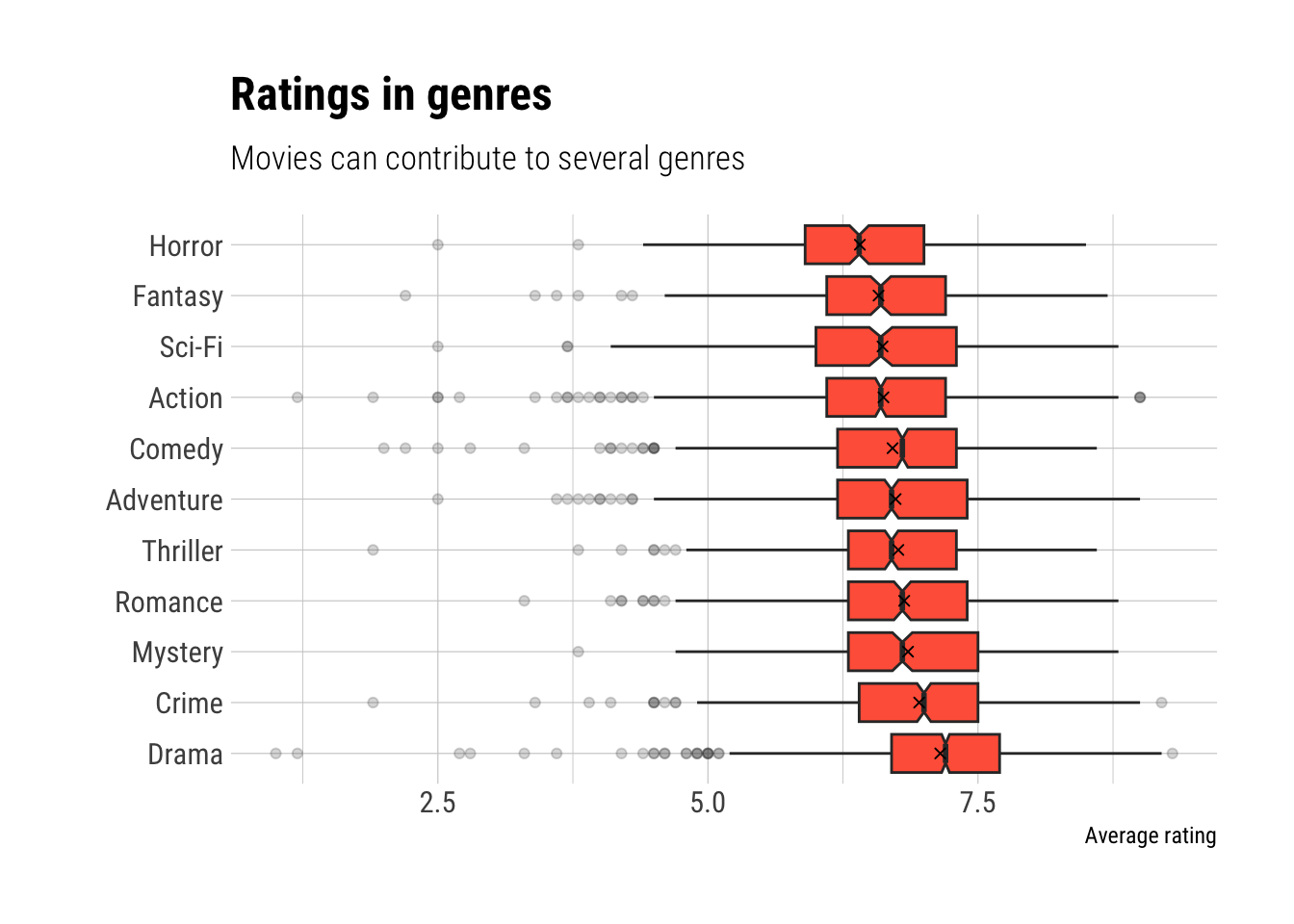
So, people seem to be especially fond of dramas. Maybe, a mistery-crime drama would be something like a perfect movie? Guess what, we can look up some these, and I am listing the top movies in this special combination of genres (I am using the “primary” title here, not the original one):
- Jai Bhim (2021)
- Se7en (1995)
- The Usual Suspects (1995)
- Witness for the Prosecution (1957)
- L.A. Confidential (1997)
- Drishyam (2015)
- Prisoners (2013)
- Memories of Murder (2003)
- The Invisible Guest (2016)
- Mystic River (2003)
Meh, I fell asleep during L.A. Confidential. Also, I did not enjoy Mystic River very much, but that might be just me.
There is a lot more that could be done with the IMDb dataset - maybe I’ll come back to it in a later post.